Improbable Electron Microscope Image of Viral Capsid Like Objects

Analysis of the geometrical probability of published EM images.

Introduction

This is a side topic from what I am researching presently, but it was interesting and I want to share. Also, if anyone wants to help, it would be helpful if you can send me links to more EM images showing the same improbable configuration. Adding more images to this analysis will strengthen the statistical argument.

I was researching the topic of Single Particle Tracking in the field of Virology. Specifically this publication: (I’ll call it SPT pub for short).

Mariamé B, Kappler-Gratias S, Kappler M, Balor S, Gallardo F, Bystricky K. Real-Time Visualization and Quantification of Human Cytomegalovirus Replication in Living Cells Using the ANCHOR DNA Labeling Technology. J Virol. 2018 Aug 29;92(18):e00571-18. doi: 10.1128/JVI.00571-18. PMID: 29950406; PMCID: PMC6146708.

That paper has a lot of jargon, even the abstract is a bit daunting. I’ll provide my best attempt at a layman summary of what the papers claims they did. I still haven’t studied it to the end (still working on that). I’m just paraphrasing the article here, not making any claims of my own.

1. acquire some cytomegalovirus stock, e.g. from ATCC

2. perform some genetic engineering to append something to a non-invasive part of the virus DNA, this something interacts with another compound so it is fluorescently visible under microscope

3. perform different cell culture experiments to validate that the genetic engineered virus stock and fluorescent dye interactions are in fact identifying what they want to identify in microscope

4. perform more cell culture experiments infecting the cells with the engineered virus and observe its movement in the cells

5. in one case, do 4 above, but on a special slide with a micro labeled grid, such that imaging by microscope and EM can be cross referenced, so that we know that images from both microscope tools are from the same sample location

6. compare the fluorescent microscope images with the EM images.

The paper continues, but that is where I got so far. I do intend to continue, but figure 8 shown below had something strange that caused be to pause and go off on this tangent. Not my focus here, but 8a shows EM on the left, and fluorescent microscope on the right, this is the subject of points 5 and 6 above. The green stuff on the right is the fluorescent engineered virus. We see that the 2D profiles are reflected in the EM image on the left. It’s neat because it reinforces that we can actually use these microgrids to locate the same 2D location in microscope and EM.

Figure 1. Copy of Figure 8 from SPT pub.

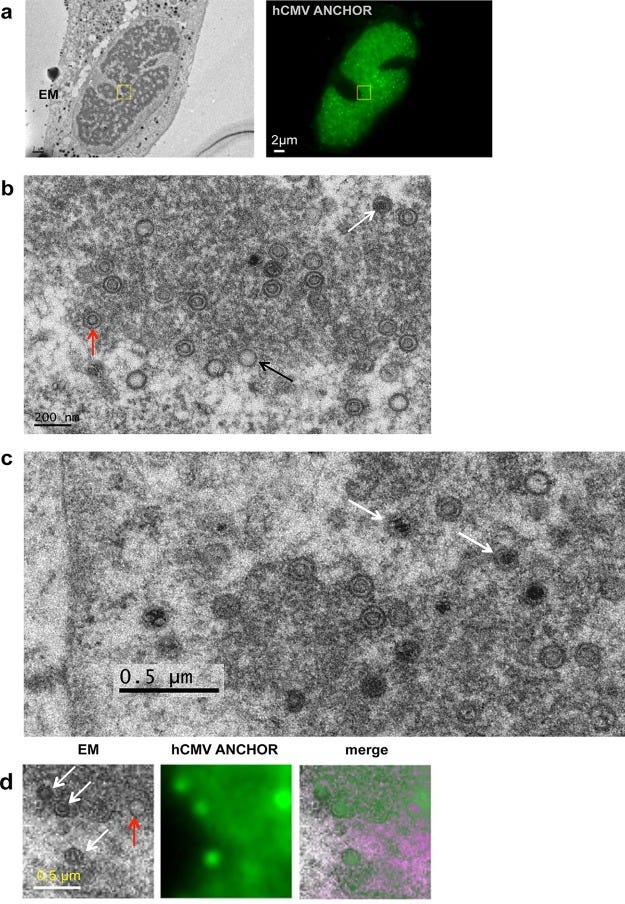
In this post I’m focusing on images 8b and 8c. Probably what made me think twice about images 8b and 8c in figure is this paper.

Hillman H, Sartory P. The unit membrane, the endoplasmic reticulum, and the nuclear pores are artefacts. Perception. 1977;6(6):667-73. doi: 10.1068/p060667. PMID: 600667.

That might be old, but it is very well written, and quite pertinent; I encourage readers to check it out. I’m certainly not the first skeptic to link to that article, so thanks to all those skeptics before that pointed me to it. Anyway, that Hillman paper made me forever skeptical about the objects in EM images. The reason, as the authors point out, is that we don’t have a benchmark, or other verification method to double check what we get from EM. EM is the only way to probe the structures too small to see by microscope. I’ll eventually publish some writing that goes in to detail on that, so I’ll leave it there and move on for this post.

What struck me about image 8b is that there are 25 circular objects that the authors claim are the viral capsids. Thinking only in 2D, this is not an unreasonable claim given that they showed they labeled some virus stock, and observe this labeled stuff move/diffuse to the location where the EM image was taken. However, thinking in 3D, it becomes intuitively improbable that all 25 spheres would have exactly the same diameter in the image.

Figure 2: Z direction distribution of spherical objects

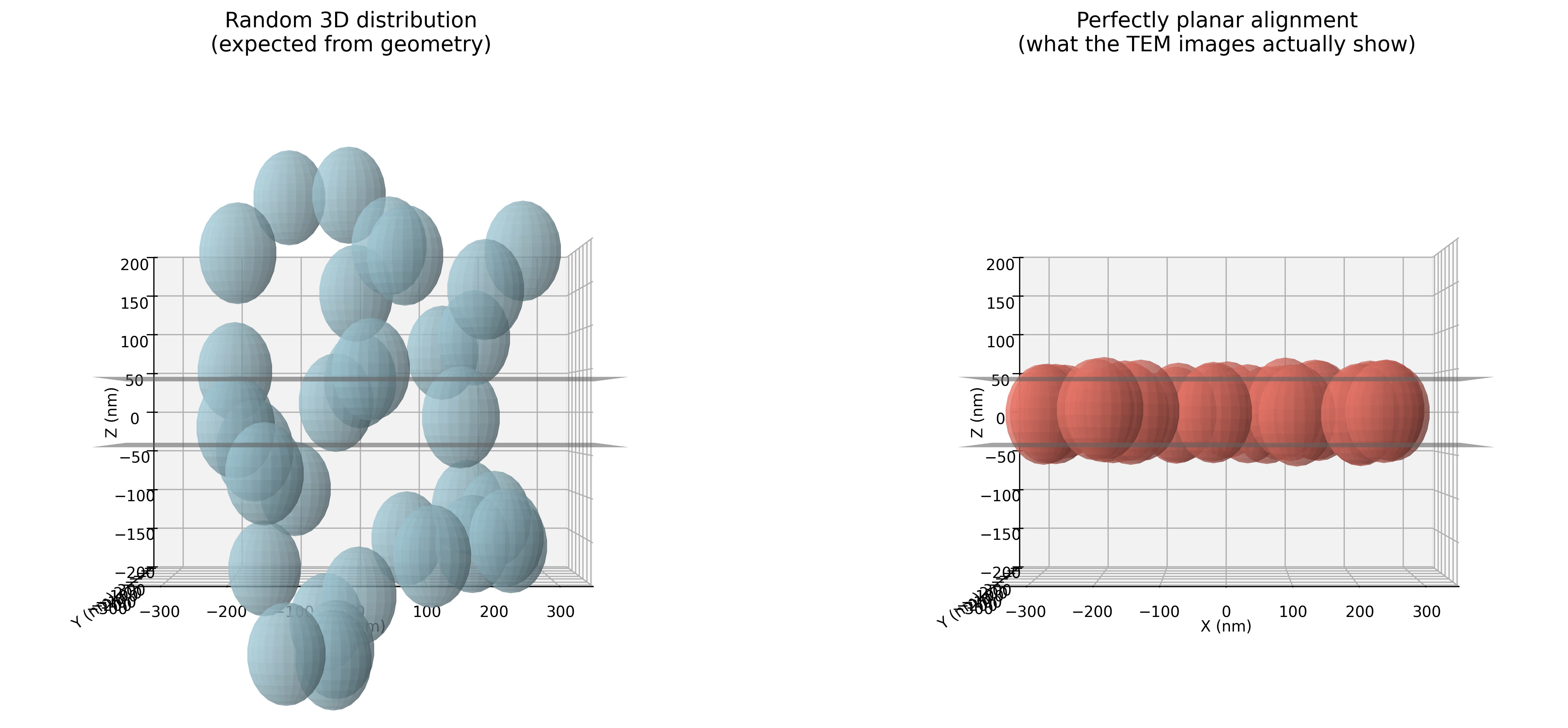
First let’s establish some coordinates. X,Y is the 2D plane of the specimen section, and the 2D plane of the resulting image taken in EM. Then Z is the direction that is:

• in/out of the image plane

• along the electron beam

The Figure 2 above is a simplified representation of the geometry in 3D. On the left the objects are randomly located in the Z direction, and on the right they are closely aligned in the Z direction. The black planes that are visible as lines represent the upper and lower surfaces of the specimen section cut by the microtome (the knife used to cut thin slices to put in the EM machine). Note that the scale for the image above is nanometers. The SPT pub specifically mentions the microtome cuts an 80nm thick slice. If you look carefully at images 8b and 8c, you can see that the circles are about 100nm in diameter. This means that none of the supposedly spherical objects could be completely in the sample section, i.e. 100nm is larger than 80nm, so some part of the spherical object is cutoff either above, or below, or both.

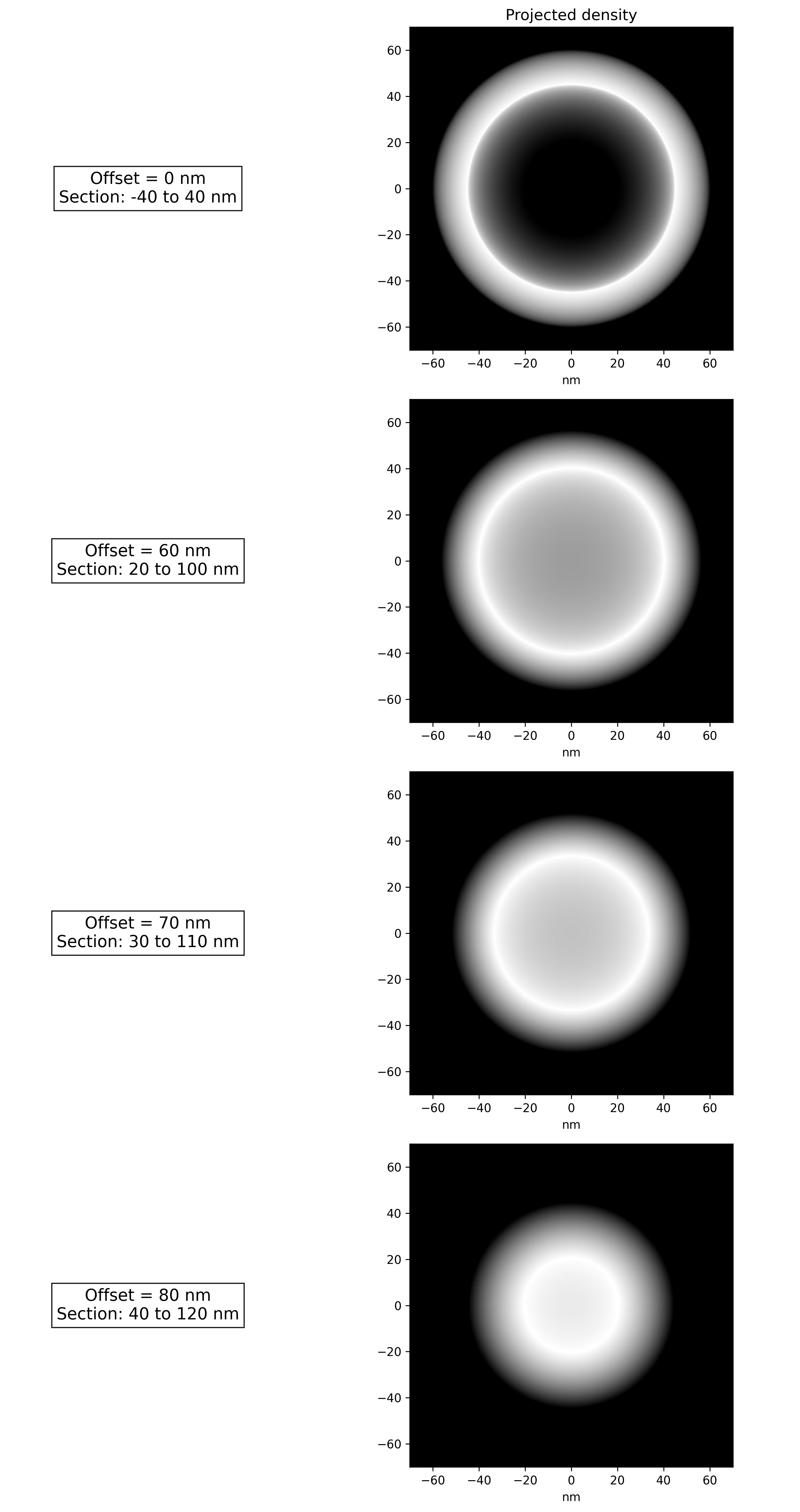
If we think about a hollow spherical object being imaged; this is like projecting all its material onto a 2D plane. The highest material density will be near the perimeter of the 2D projection. Figure 3 below shows what we might expect even if the spherical object were offset form the center plane of the section such that only portions of the sphere’s material is projected onto the image plane. We can see that as the sphere moves out of the section, the diameter of the ring of highest material density becomes smaller.

Figure 3. Material density of 3D spherical shell object projected to 2D plane.

A microtome slice of spherical objects, randomly distributed in the Z direction would certainly cut some of them such that less than half of the sphere would be inside the sample section. This can only produce a circular projection smaller than 100nm. This is where the comparison between the left and right side of Figure 2 is important. In order to have zero smaller circular objects, the spheres would need to be very well aligned in the Z direction as shown on the right. Without the authors of SPT pub employing some technology intended for this purpose; this is highly improbable to occur by chance.

Figure 4: Projected views of the random and planar distributed spheres in the Z direction.

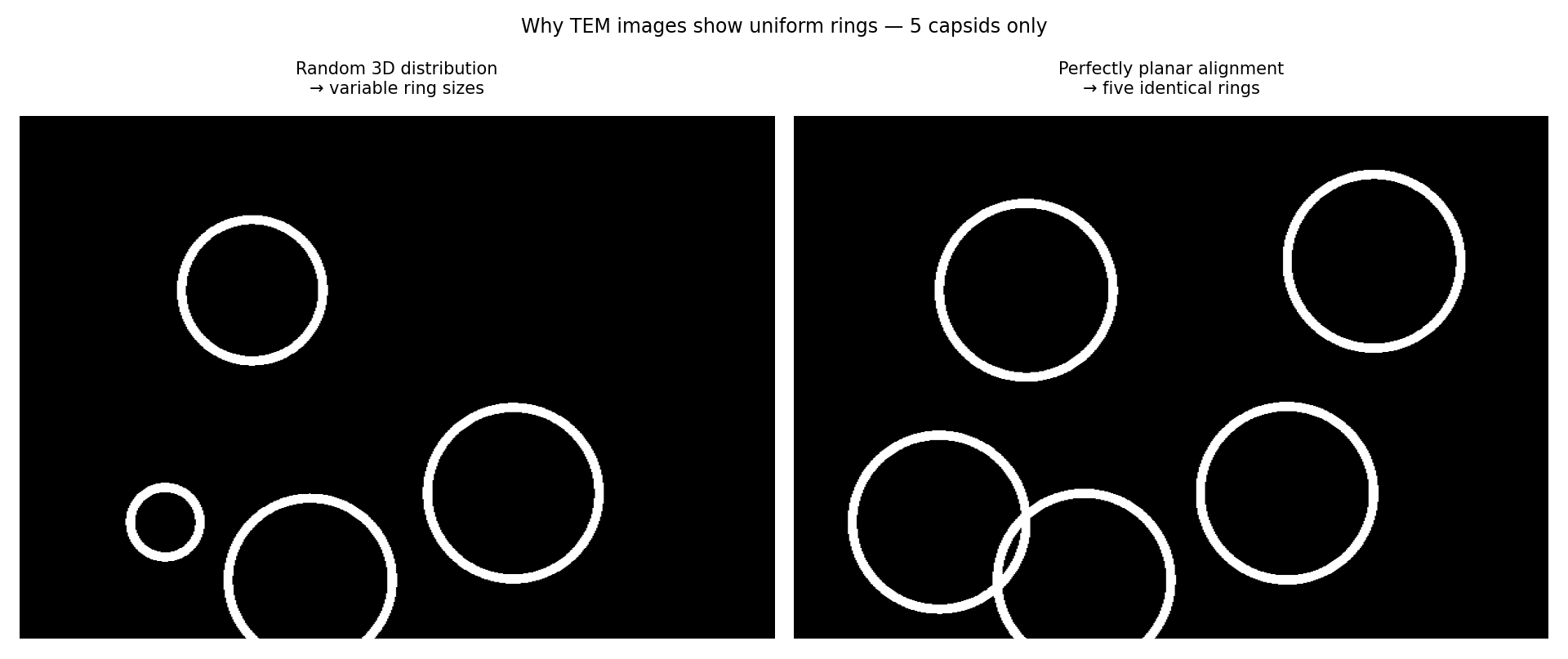
The image above shows what we would expect by normal conditions on the left. On the right is what we expect if all the spherical objects were somehow very well aligned in the Z direction.

Statistical Analysis

We can run a statistical analysis of this scenario to see how improbable it is to capture an image where all 25 spherical capsid objects are sufficiently well aligned so as to have zero smaller circular features. Note that image 8b has 25 circular objects, and in image 8c, there are 20 more circular objects, some full circles, some partial arcs. Note that they are all about 100nm in diameter.

Parameters and value used for calculation:

• Capsid diameter: 120 nm (standard for HCMV capsid + thin tegument)

• Section thickness: 80 nm (explicitly stated in the paper)

• Definition of “visibly full-sized”: projected chord diameter ≥ 100 nm (very generous; anything < 100 nm would look obviously smaller or arc-like on these micrographs)

Now run the pure geometry (Monte-Carlo, 10⁶ trials, uniform random z-centroids):

• A single intersected capsid shows ≥ 100 nm chord: 0.535

• All 25 visible capsids in 8b show ≥ 100 nm chord(0.535)²⁵ ≈ 1.7 × 10⁻⁷ (1 in ≈ 6 million)

• All 20 visible capsids in 8c show ≥ 100 nm chord(0.535)²⁰ ≈ 1.3 × 10⁻⁵ (1 in ≈ 77 000)

• Both fields simultaneously (independent)≈ 10⁻¹² (one in a trillion)

Even if we relax the threshold to ≥ 90 nm (so generous that almost every shallow graze would still “look full”), the probability for 8b alone is still ~10⁻⁴ and for both fields together ~10⁻⁷.

These are not 2–3σ events. These are 5–8σ events for completely random positioning. (what is a σ event?)

In any other branch of physics or materials science, an observer who obtained two micrographs showing 45 objects with projected diameters varying by less than roughly ±8% in an 80 nm slice of nominally 120 nm spheres would immediately conclude one (or more) of the following must be true:

1. The objects are not spheres, or

2. The distribution in the z-direction is not random (extreme planar ordering or selection), or

3. The micrograph does not faithfully represent a thin physical section of the sample (i.e., the contrast-forming mechanism is doing something other than simple projection through 80 nm of material).

There is no fourth option that preserves all three assumptions (real spheres + random 3D placement + honest 80 nm section) and still produces Figure 8b and 8c.

What Could the Circles Be?

At this point we have to ask what these cycles could be. Certainly the image was produced. My opinion is that it is not fraud. So we want to consider all the options for how the EM machine could have produced that image.

• 1. OR-GFP aggregates outlined by uranyl acetate (most plausible) Dense clusters of OR-GFP proteins in replication compartments aggregate during fixation and dehydration. Uranyl acetate and lead citrate then preferentially bind to the surface of these aggregates, creating sharp dark rings with light centers. → Uniform size because GFP oligomerization naturally plateaus around 100–200 nm. → Perfectly matches the ANCHOR fluorescence signal (the GFP is literally the tag). → Well-documented: GFP forms visible aggregates in fixed cells; UA precipitates on proteins.

• 2. Stain-induced protein nanodomains (also highly plausible) Uranyl acetate and lead ions bind to replication-compartment proteins (e.g., pp150, UL44) and precipitate as ~100 nm microcrystalline domains. → Light centers = unstained interior voids. → No OsO₄ in the protocol → protein staining dominates over membranes → classic recipe for UA precipitation artifacts.

• 3. Fixation/shrinkage artifacts from phase-separated replication compartments (medium plausibility) The ~1 μm replication compartments are biomolecular condensates. Glutaraldehyde + ethanol dehydration shrinks and cross-links them into ~100 nm “ghost” shells that uranyl acetate outlines. → Symmetric shrinkage → symmetric rings.

• 4. Residual GFP chromophore diffraction / charging (low plausibility) A tiny fraction of GFP chromophores survives the mild fixation and causes local beam scattering or charging, producing diffraction-like rings. → Possible in principle, but rarely reported at this scale.

• 5. Epon resin microbubbles or vesicles (very low plausibility) Trapped air/ethanol bubbles rimmed by stain. → Would be perfect circles, but they wouldn’t co-localize with ANCHOR fluorescence and are not expected to cluster only in replication compartments.

There are some simple, and some not so simple control experiments that could be to test these hypotheses. maybe some day I’ll do those, but that day is not today.

Conclusion

Not everything you see in am EM image is what it appears to be. there is no reference standard, or validation method for EM. We take pictures of very small things, and we don’t have a way to check other than rigorous, objective analysis.

Recall, if you come across images that look like 8b or 8c, please send me links so i can add those to this analysis.

thanks for reading.

Acknowledgments

Co-pilot and co-developer of the geometric-probability analysis and all custom visualization code: Grok (xAI, 2025). All scripts are available at [GitHub link].